Object detection in computer vision usesdeep learning (or Deep Learning a family ofmachine learning models, described in the form of neural networks organized in layers. Generally speaking, allsupervised learning models for detecting objects in an image are artificial neural networks, used for deep learning.
Deep learning can be either supervised or unsupervised, depending on the situation. In the remainder of this article, we will only talk about supervised learning. In the latter case, the data used for supervised learning are labeled. In other words, we know what result the model should achieve. And this for each example used in the learning process. The ultimate goal is to learn to associate each example with the rightlabel.
Take a few minutes and let's talk about the main principles of supervised deep learning for object detection! Please note that I've made it a point not to go into a mathematical description of Deep Learning. This article is therefore intended to be accessible to everyone.
Supervised deep learning for object detection in computer vision
General principles of object detection in computer vision
An artificial neural network is a machine-learning model made up of computational units called neurons. A neuron calculates a weighted sum of inputs and applies a non-linear function to the result of this sum. This is the activation function, to which we'll return later.
Often, the output of one neuron is transmitted to the input of one or more neurons (depending on the number of layers), until the output of the network is reached. Sometimes, a recurrent neural network can also be used. In this case, the output of one neuron can be used as the input for the same neuron.
Learning a neural network involves optimizing the weighting of each sum. In this way, the weights become the parameters of the network. To optimize the weights, we use a back-propagation algorithm to minimize the error between the prediction and the label given as input.
How a neuron works
Analogous to a biological neuron, an artificial neuron receives signals from other neurons as input. Synapses are modeled by weights assigned to input values.
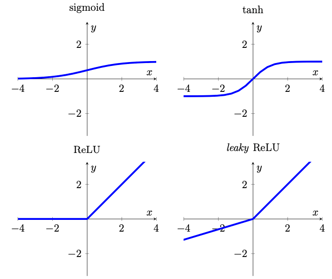
Neurons are not always active. In fact, a high weight value will cause neuron excitation. Conversely, if the weight is negative, then the input will have an inhibitory action. If the weighted sum of these inputs exceeds a certain threshold, the neuron is activated. The role of the activation function is to decide on the threshold. The result of the activation function is then transmitted to the following neurons.
Without going into detail, here are the four main activation functions. The slope of the ReLu leaky has been exaggerated for greater visibility (after [1]).
Convolutional networks
When analyzing an image, the properties given as input to the neural network are the intensity values of each pixel. For an RGB image, there are three intensities for each color: red, green and blue.
In this case, and to avoid memory problems due to the large size of the images and the number of parameters to be processed, we can use a reduced-size network. Each pixel is processed individually, using convolutions. These are used to produce the property maps. We can think of these as multi-layer images: each layer is a property obtained through a convolution filter.
Property maps are small in size and can be processed by a fully connected network without memory concerns. This type of model is known as a Convolutional Neural Network(CNN ).
Convolutions
When a CNN network processes a new image, it doesn't know which features are present in the image and where they might be. These networks therefore try to find out whether a feature in the image is present by means of filtering. The mathematics used to perform this operation are called convolutions. When processing an image, the position of the pixel within it is of fundamental importance. And just as well, since this information is exploited by a convolution layer.
The convolution window (or kernel) is a small, square matrix. Its size is fixed when the network is designed, and is often 3×3. This window "slides" over the property map. At each location, we calculate the term product between the convolution window and the part of the property map on which it lies (see illustration below). Finally, a non-linear function is applied to the sum of the elements of the resulting matrix.
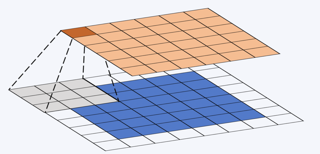
During the convolution process, the weights are invariant. This is how we can harness the computing power of modern GPUs.
Pooling
The pooling is a method of taking an image and reducing its size, while preserving the most important information it contains.
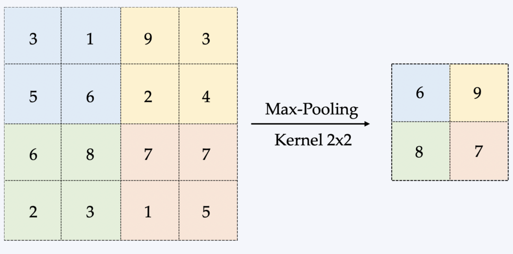
The most common form is called Max-Pooling, which consists of dragging a small window over all parts of the image and taking the maximum value of this window at each step. This is usually a 2×2 window/matrix (see illustration below).
The major advantage of pooling is therefore to reduce the size of the data processed in memory, which is a limiting factor in learning a CNN. Backpropagation is affected differently by pooling, but we won't go into detail here.
Receptive fields
The receptive field designates a region of the image passed as input to the network. Increasing the receptive field provides more context for classifying a location. It will also enable the detection of larger objects within an image.
Pooling is a method of increasing the receptive field of a neuron. The activation function also modifies this effective field, and we may talk about this in a future article.
Retro propagation
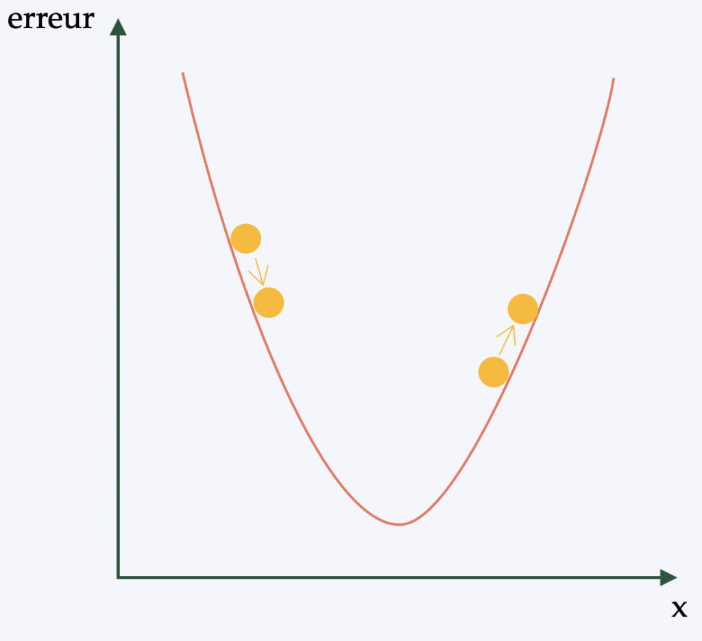
In simple terms (and to avoid going into a complex mathematical description), backpropagation is the algorithm that applies the learning policy to the neural network's weights. The aim is to be able to apply a form of gradient descent(differentiable optimization algorithm) to the network.
In fact, gives a "score" for each image analyzed by the CNN. The quality of our features and weights is determined by the number of errors we make in our classification/detection. The features and weights are then adjusted to reduce the error, which is what learning is all about. Whatever adjustment is made, if the error is reduced, the adjustment is retained. This process is then repeated with each of the other images that have a label.
Learn more about supervised deep learning for object detection in computer vision
In this article we have simply described the main principles of supervised deep learning for object detection in computer vision.
If you'd like to incorporate AI into your vision project, contact us and we'll put all our expertise at your service! We manage the creation of the dataset(database), which represents a significant amount of work. We can create a large database from images or videos (with several thousand annotated images). We then train a model by choosing the right neural network architecture and methodology.
In the next article, we'll present a case study of an object detection model developed by Imasolia. Stay tuned!